
Talk To Us
Radically accelerate your roadmap with Tangram Vision's perception tools and infrastructure.
Thank you! Your submission has been received!
Oops! Something went wrong while submitting the form.
Radically accelerate your roadmap with Tangram Vision's perception tools and infrastructure.


Table of Contents
If the word “optimization” brings back old memories of pulling an all-nighter for an AP Calc exam… take a deep breath and let’s focus on something sweeter. The fundamentals of optimization are actually quite simple and we’ll use ice cream to illustrate.
In my own words, optimization is simply “making the choice that is best.” Let’s imagine a set \(X\) filled with choices. Let’s say this set \(X\) is a set of ice cream flavors \({ \text{mint chocolate chip}, \text{rocky road}, \text{pistachio}}\).
While you might be tempted to choose your favorite flavor, we haven’t finished setting up the optimization problem yet. For the optimization problem, we need context. This context is given by a function \(f: X \to Y\) where \(Y\) is a totally ordered set. With this example, we could define \(f\) as being the function representing your four year old niece’s ranking of these flavors. You ask your niece to rank these ice cream by assigning the numbers \(Y = \{1, 2, 3\}\) (with 1 representing the best), and she says:
$$\begin{aligned}&f(\text{mint chocolate chip}) = 1 \\&f(\text{rocky road}) = 2\\&f(\text{pistachio}) = 3\end{aligned}$$
In this case, it’s trivial to see that mint chocolate chip is the “best” choice.
While it would be great to have a niece available any time to provide trivial solutions to optimization problems, in reality, we almost always need to do this work ourselves. Therefore, we need to understand how to set up an optimization problem so that we can find our solution. Formally, an optimization problem can be defined as:
Given a function \(f\) mapping a set \(X\) to totally ordered set \(Y\), find the best \(x^{*} \in X\), where best is defined by \(f\) so that \(f(x^{*}) \leq f(x)\) for all \(x \in X\).[1]
This statement is quite verbose and mathematicians value brevity, so it’s common to see the above problem rewritten as
$$\text{minimize}\ f(x)$$
and the best choice \(x^{*}\) is typically written as
$$x^{*} =\text{argmin}_x f(x)$$
or, in words, the argument which minimizes the function \(f\).
💾 There is nothing special about our choice of inequality ≤ in the above definition. Many books on optimization will use the convention ≥, \(\text{maximize}\) and \(\text{argmax}\) to define their optimization framework. Here, we note that the choice does not affect generality since there is a canonical transformation \(f \to -f\) such that \(f(x) \mapsto -f(x) \ \forall x\) which changes minimization of \(f\) to maximization of \(-f\).
You may have noticed the use of the word “find” in our definition of an optimization problem. In many ways, optimization can be thought of as a search problem, with the objective of finding that best choice: \(x^{*}\). In our ice cream example, we humans (incredibly adept at quickly remembering up to nine numbers), very easily find the best choice. However, if we visited Baskin Robbins, the size of the set \(X\) would increase to 31 flavors and we would find it more difficult to quickly identify the best flavor. Are we doomed if we expand our set of choices to an infinite number of possibilities (e.g. \(X = \mathbb{R}\))? [2]
Since exhaustively comparing all choices is infeasible, we need to find a way to limit our search space. Calculus provides us the tools to do just that.
For this section, we’ll assume that \(f\) is a real-valued function defined on real number choices (\(f: \mathbb{R} \to \mathbb{R}\)). We’ll further assume that this function is twice continuously differentiable (\(f\) is of class \(C^2\)).[3]
Since this blog post is not a rigorous course on analysis or optimization, we’ll accept without proof that if \(x^{*} = \text{argmin}_x f\), then we must have that \(f'(x^{*}) = 0\), or in other words it must necessarily be true that \(f'(x^{*}) = 0\).[4]
In single-variable calculus, this fact is used in the first derivative test. The formal version of this statement is called The First-Order Necessary Condition. The astute reader will note that condition assumes that we already know \(x^{*}\), which seems less useful given that we are looking for that exact value! However, we can use this condition to restrict our search space and (hopefully) simplify our problem to evaluating a handful of choices.
As such, we define a critical point to be any \(x \in \mathbb{R}\) such that \(f'(x) = 0\). As an example, let’s take \(f(x) = x^2 - 4x + 7\).

Solving for \(f'(x) =0\), yields the set of critical points \(\{2\}\). Take a moment to appreciate what we’ve just done. With a little bit of calculus and algebra, we’ve pruned our set from an infinite number of possibilities to just one. So \(x^{*} = 2\) since it’s the only option, easy enough, right?
Unfortunately, there’s a bit more complexity here. So far in the post, we’ve a priori assumed the existence of an \(x^{*}\). As a counterexample, consider the function \(f(x) = -x^2 + 4x - 7\).
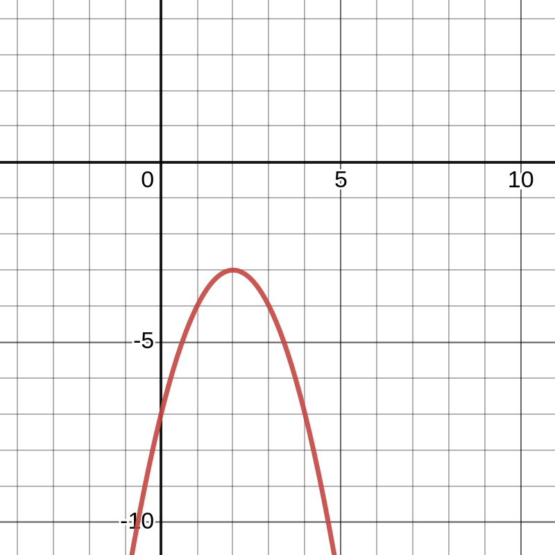
This function has the same critical points and the previous function, but this function has no minimum. In short, we’ve replaced our original problem — search the entire space and find the minimum — with a new problem: decide which (if any) of our critical points is the minimum. In order to solve this new problem, we have to take a brief detour and understand locality.
Looking at the definition of the derivative in single variable
$$f'(x) = \text{lim}_{h \to 0} \frac{f(x + h) - f(x)}{h}$$
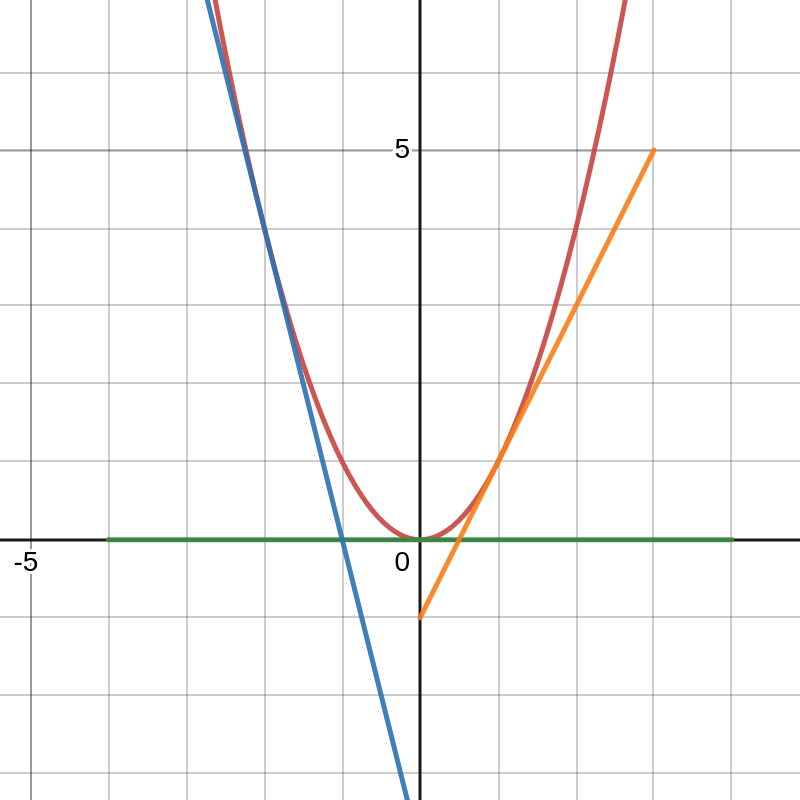
we realize that this operation only describes our function “close to” to the point in question.[5] Thus, differential calculus only describes local behavior of a function. To leverage the strengths of differential calculus, we define a concept of local minimum. To distinguish from the global minimum \(x^*\) we will denote our local minimum as \(x^{*}_l. \) We say that \(x^{*}_l\) is a local minimum of \(f\) if \(x^{*}_l\) is a minimum when we only look at points “close to” \(x^{*}_l\).[6] As an example, consider the function \(f(x) = x^4 - 3x^3 + x^2 + x + 1\) shown below.
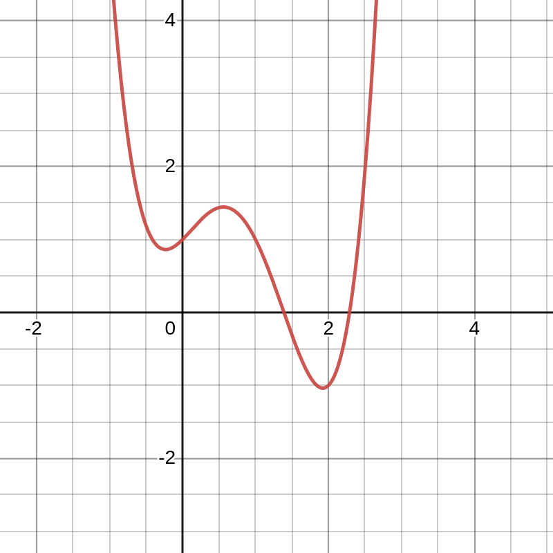
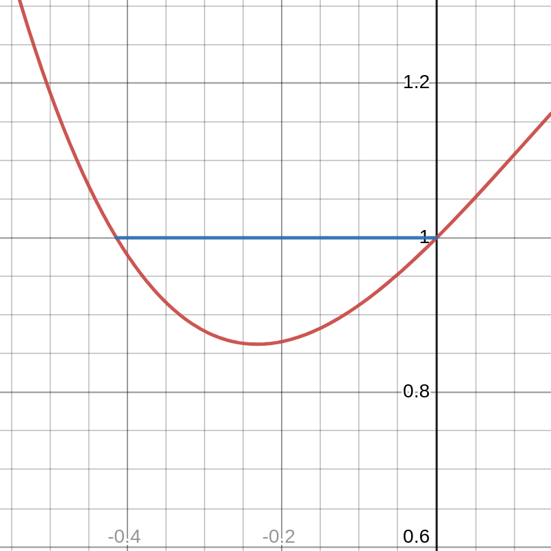
It is easily seen that this graph has two local minima. If we zoom in and look at the function “close to” the first local minimum, we see
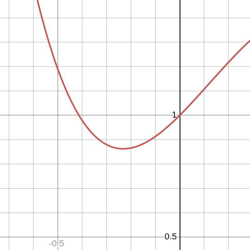
and in this region, this local minimum appears to be the only minimum.
We should restate the First-Order Necessary Condition with this knowledge. If \(x^{*}_l\) is a local minimizer of \(f\), then we must have that \(f'(x^{*}_l) = 0\). A corollary to this statement would be that our local minimizers can only occur at our critical points (as defined above). For clarity, we will rename our \(x^{*}\) as the global minimizer. This leaves us with a few questions
The answer to these questions lies in an understanding of convexity.
My favorite definition of convexity is a geometric one. Put simply, a function \(f\) is convex if the line connecting any two points on that function lies above the function between those two points. Since this is a geometric definition, it’s most easily understood geometrically as shown in the graph below.[7]
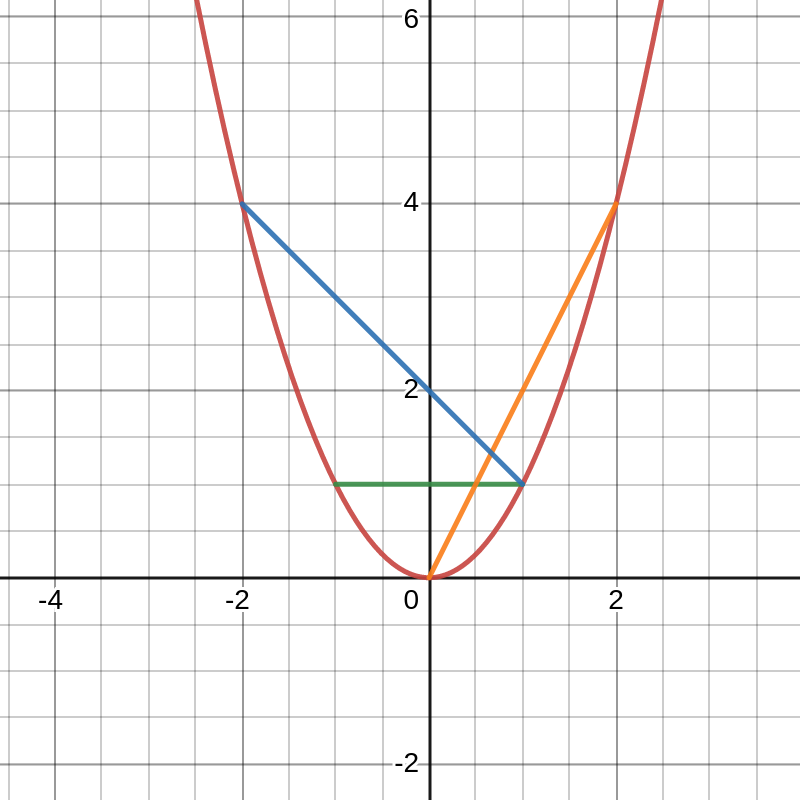
As seen, every line lies above the function. A consequence of convexity for differentiable functions is that tangent lines must lie below the function as shown in the graph below.
In particular, a convex function must lie above all of its tangent lines with a slope of 0. Points where the tangent line is 0 are precisely the critical points we’ve identified with our First-Order Necessary Condition. In short, if we have a critical point for a convex function \(f\), then that critical point is our global minimum \(x^{*}_l\). Once again, we’ve moved the goal-posts. Now, we must determine whether our function \(f\) is convex.
Fortunately, calculus saves the day once more. We’ll state without proof here that if \(f''(x) > 0\) for all \(x \in \mathbb{R}\) then the function \(f\) is convex. In some cases, this can be shown easily (e.g. \(f(x) = x^2\)). In other cases, this is not so easy to show and the exhaustive approach of testing every \(x\) is infeasible. It turns out that convexity is a strong assumption. This is precisely why such strong implications follow from convexity.[8]
As such, we’ll relax our assumption of convexity and define a function to be locally convex around a point \(x\) if \(f''(x) > 0\). Again, this uses the same notion of “close to” as we used in the previous section. As an example, we will again use \(f(x) = x^4 - 3x^3 + x^2 + x + 1\). From the graph, we can see that this function is locally convex and evaluating the second derivative at that critical point gives a positive value.
This insight allows us to state the Second-Order Sufficient Condition: If \(x^{*}_l\) is a critical point of \(f\) and if \(f\) is locally convex around \(x^{*}_l\) (i.e. \(f(x^{*}_l) > 0\)), then \(x^{*}_l\) is a local minimizer of \(f\).[9]
In short, to optimize a function, we can find the critical points using the First-Order Necessary Condition and then classify them as local minima using the Second-Order Sufficient Condition. If we can additionally show that our function is globally convex, then we have found a global minimum.
There are situations where we need to make multiple choices to find the minimum of a function. Such functions are defined on a vector space and denoted \(f: \mathbb{R}^n \to \mathbb{R}\). Fortunately the optimality conditions we’ve listed above have natural extensions to multiple variables. For brevity, we’ll state them here and refer the reader to a book on real-analysis and optimization for further insight. [10,11]
First-Order Necessary Condition
If \(\mathbf{x}^{*}_l\) is a local minimizer of a \(C^1\) function \(f\) then the gradient of the function \(\nabla f(\mathbf{x}^{*}_l) = \mathbf{0}\).
Second-Order Sufficient Condition
If \(f\) is a \(C^2\) function with a critical point \(\mathbf{x}^{*}_l\) ( \(\nabla f(\mathbf{x}^{*}_l) = \mathbf{0}\)), and \(f\) is locally convex (the hessian \(\nabla^2 f(\mathbf{x}^{*}_l)\) is positive definite at \(\mathbf{x}^{*}_l\)) then \(\mathbf{x}^{*}_l\) is a local minimizer of \(f\).
Additionally, if \(f\) is globally convex (the hessian \(\nabla^2 f(\mathbf{x})\) is positive definite for all \(\mathbf{x} \in \mathbb{R}^n\)) then \(\mathbf{x}^{*} = \mathbf{x}^{*}_l\) and \(\mathbf{x}^*\) is a global minimizer of \(f\).
In this brief introduction to the theory of optimization, we were able to touch on a lot of important points. However, there are many nuances and sub-fields of optimization we aren’t able to address in this short blog post. There are theories of discrete optimization, constrained optimization and even optimization on non-flat spaces (manifolds).
During this introduction to optimization, we’ve been a bit cavalier regarding the simplicity of finding critical points. If you go back and look carefully, algebraic techniques have been doing a lot of heavy lifting to help us find these critical points. Most equations are not easily solved algebraically and identifying closed-form solutions can be impossible. [12]
This leads us to solutions from the rich and interesting field of numerical optimization. We will cover standard numerical optimization techniques, applications and examples in a future post.
Optimization problems are ubiquitous in many fields - not just ice cream choices. At times, this is obvious from naming such as in maximum likelihood estimation and maximum a posteriori estimation. However, optimization appears in many applications — inverse kinematics, trajectory planning, and deep learning, just to name a few.
At Tangram Vision, we see multi-sensor, multi-modality calibration as an exciting and difficult optimization problem. To learn more about calibration as an optimization problem, check out our series Calibration From Scratch Using Rust — but if you’d rather eat ice cream and have us work through the mathematics of how to calibrate your sensors, get in touch.
[1] Given this definition, \(x^{}\) may not be unique. If \(f\) is not injective, there may be multiple minimizers. In this post, for simplicity, we will assume that \(x^{}\) is unique.
[2] Here we intentionally omit the interesting and beautiful field of discrete optimization. The curious reader is encouraged to learn more about integer programming and combinatorial optimization. As such, the usage of “infinite” in this post should have the interpretation of uncountable.
[3] This and the following sections have natural extensions to a function \(f: B \to \mathbb{R}\), where \(B\) is a connected and compact subset of \(\mathbb{R^n}\). Such optimization problems can be posed as constrained optimization problems and solved using the KKT conditions. In this post, we will assume an unconstrained optimization problem.
[4] For a rigorous treatment of calculus we refer the reader to Stephen Abbott’s Understanding Analysis, or for more self-induced math torture any of Walter Rudin’s books will do.
[5] This notion of “close to” is made rigorous in most books on real analysis.
[6] In other words, \(x^{}_l\) is a local minimizer of \(f\) if there exists an open subset \(U \subset \mathbb{R}\), such that \(x^{}_l \in U\) and \(x^{*}_l\) is the minimizer on the function \(f\) restricted to \(U\), typically denoted by \(f\vert_U\).
[7] Technically, such a function \(f\) is strictly convex. Non-strictly convex functions allow for intersections with the line at points other than the endpoints of the line. For simplicity, we’ll restrict the discussion to strictly convex functions in this post.
[8] Because convexity is so powerful, we sometimes jump through many hoops to make an optimization problem convex. This process of making an optimization problem convex is called “convexification.” A particularly impressive example of convexification is SE-SYNC.
[9] There is also a Second-Order Necessary Condition, which addresses non-strictly convex functions.
[10] Yes, there is a lot of nuance here that we are glossing over. For example, optimization over infinite dimensional vector spaces, topological completeness, and optimization on manifolds.
[11] Notation of derivatives is inconsistent as you get into higher mathematics (especially in the study of differential geometry). For this section, I chose the notation that most people should be familiar with from multivariable calculus.
[12] For more insight, explore Abstract Algebra and Galois Theory.