
Talk To Us
Radically accelerate your roadmap with Tangram Vision's perception tools and infrastructure.
Thank you! Your submission has been received!
Oops! Something went wrong while submitting the form.
Radically accelerate your roadmap with Tangram Vision's perception tools and infrastructure.


Table of Contents
So, you’ve purchased an IMU for a couple bucks and you’re not sure how to do anything useful with it? Your IMU state estimates seem to fly off beyond the horizon leaving you wondering what good is an IMU? You can’t seem to figure out how to read an IMU datasheet — I mean what is a \(\sqrt{Hz}\) anyway? It seems like you either have to hire an expert state-estimation engineer or pay thousands of dollars for a tactical-grade IMU?
Well, you’ve come to the right place. We are here to cure all your IMU woes and provide some insight into these confusing sensors. In this five part blog series, we’ll cover
If you’d like to be notified of when that next post drops, just follow us on LinkedIn, X, or subscribe to our newsletter. Don't have an IMU yet? Consider pre-ordering our upcoming HiFi depth sensor, for high-resolution 3D sensing...with a built-in IMU!
In our last post, we talked about how to model the stochastic error of an IMU’s accelerometer and specific force signal. We presented a noise model composed of three components and a power spectral density given by
\(S_{\eta}(f) = N^2 + \frac{B^2}{2 \pi f} + \frac{K^2}{(2 \pi f)^2}.\)
However in our last post, we assumed that these coefficients \(N, B, K\) were given in the IMU data sheet. What can we do if these values are not given to us? One approach would be to analyze the power spectrum of your IMU and fit a model to find the coefficients. The most commonly used tool, however, is the Allan Variance.
The Allan Variance (AVAR), is a statistical tool used originally used for quantifying the stability of oscillating clocks. It is a time-domain analysis technique and, as such, is fairly easy to interpret and calculate. First, we’ll walk through the calculation of the Allan Variance and then discuss its utility in characterizing IMU noise.
To calculate the Allan Variance of our noise signal \(\eta(t)\) we first approximate the slope between samples taken \(\tau\) seconds apart
\(y_i(\tau) = \frac{\eta((i + 1) \tau) - \eta(i\tau)}{\tau}.\)
Then we take these approximated slope values and compute a 2 sample Bessel-corrected variance
\(z_i(\tau) = y_i^2(\tau) + y_{i-1}^2(\tau) - \frac{1}{2}(y_i(\tau) + y_{i-1}(\tau))^2.\)
Lastly, we take a scaled average over all the 2 sample variances of our approximated slope values
\(\sigma^2_\eta(\tau) = \frac{1}{2N} \sum_{i = 0}^N z_i(\tau)\)
Here we note that that the number of approximated slope 2-sample variances is dependent upon the the duration of your input signal and the value of \(\tau\).
Now, what is this Allan Variance thing that we’ve computed and why does it make sense to compute? As seen in our computation, we’ve essentially created an estimator for the variance of the expected change per second in a duration \(\tau\). As such, the Allan Variance gives us a notion of how much we can expect the IMU noise to change at different horizons \(\tau\).
However, in dealing with any estimator, we should be cognizant of its confidence bounds. As mentioned earlier, the number of samples depends on the duration of the signal and the value of \(\tau\). As such, the confidence of our estimated Allan Variance decreases as \(\tau\) increases. To improve this confidence of our estimate for large \(\tau\), data can be sampled from the sensor for an extended period of time. It’s fairly common to collect samples from an IMU for many hours before performing an Allan Variance analysis. Also, there are ways to use sliding windows to compute the Allan Variance that are more computationally efficient and also yield lower estimator variance, but the calculation presented here should help you build intuition of the Allan Variance.
⚠️ If you’ve been reading very carefully you may say “hey! we can’t compute the Allan Variance on the noise signal because our IMU doesn’t report what part of the signal is noise!” You’re absolutely correct. In practice, the samples on which the Allan Variance are computed are collected on a stationary IMU. Collecting data in this manner means we don’t have to worry about any constant signal (like gravity) since that will be removed during the 2-sample variance computation.
In industrial settings, the Allan Variance is computed on samples taken on a vibration-isolated table, in an electrically insulated environment and at constant temperatures. This is a really good way to characterize the IMU, but in practice the noises observed during operation will have a higher noise floor than what is reported in a industrial Allan Variance analysis. As such, any values computed during an Allan Variance analysis serve as lower bound on the actual noises that will be observed during operation.
Typically, the Allan Variance will be used to calculate the Allan Deviation (ADEV) \(\sigma_{\eta}(\tau)\) as one would do with a typical variance and standard deviation. This Allan Deviation can be displayed graphically in a log-log fashion on an Allan Deviation plot, sometimes called a Sigma-Tau Diagram. An example of such a diagram is shown below.
.png)
As seen in the diagram, the Allan Deviation typically descends at low values of \(\tau\), and then has a flat region, before increasing for larger values of \(\tau\). At this point though, all we’ve done is produce a nice graph, how does this tie in to our noise model?
The Allan Variance is related to the power spectral density by
\(\sigma_{\eta}^2(\tau) = 4 \int_0^{\infty}S_{\eta}(f) \frac{\sin^4(\pi f \tau)}{(\pi f \tau)^2} df.\)
This transformation can be used to determine our noise coefficients \(N, B, K\) from an Allan Variance calculation. To show the correspondence, we will perform this integration for each term in our noise model and then use the Allan Deviation plot to estimate our noise model coefficients.
Evaluating the transformation integral for the white noise term, we have
\(\sigma^2_N(\tau) = \frac{N^2}{\tau}\)
If we take the logarithm of the Allan Deviation \(\sigma_N(\tau)\) , we have
\(\log(\sigma_N(\tau)) = \log(N) - \frac{1}{2} \log(\tau).\)
Or in words, the white noise term has a slope of -1/2 in the log-log Allan Deviation plot. Plotting the Allan Deviation of the white noise term confirms our analysis.
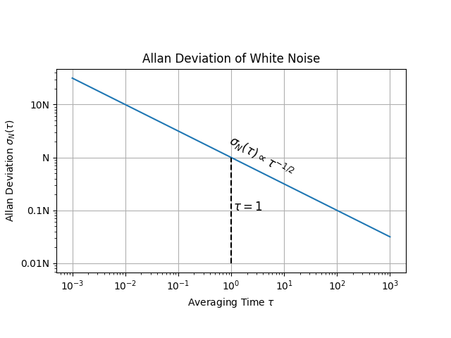
With this plot, we can “read off” the coefficient \(N\). To do so, we find the region with slope -1/2 and evaluate that line at \(\tau = 1s\), since \(\sigma_N(1) = N\).
Evaluating the transformation integral for the brown noise term, we have
\(\sigma_K^2(\tau) = \frac{K^2 \tau}{3}\)
If we take the logarithm of the Allan Deviation \(\sigma_K(\tau)\), we have
\(\log(\sigma_{K}(\tau)) = \log(K) + \frac{1}{2} \tau - \log(3)\)
Or in words, the white noise term has a slope of 1/2 in the log-log Allan Deviation plot. Plotting the Allan Deviation of the brown noise term confirms our analysis.
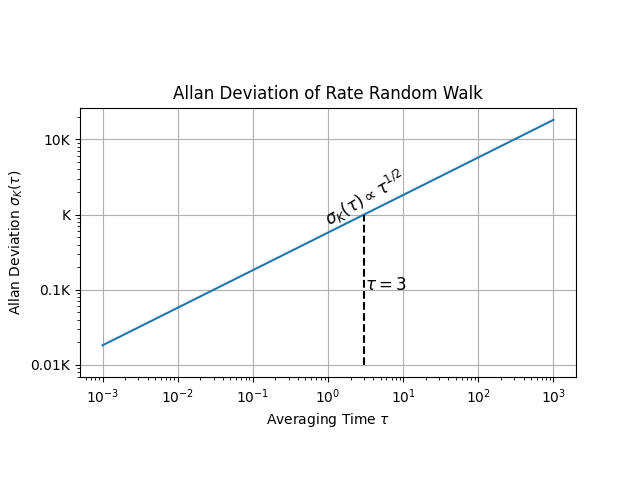
With this plot, we can “read off” the coefficient \(K\). To do so, we find the region with slope 1/2 and evaluate that line at \(\tau = 3s\), since \(\sigma_K(3) = K\).
As always, we save the tricky bias instability for last. Here, we are going to adapt our model a bit to include a corner frequency \(f_c\) above which we do not care about contributions due to flicker noise. This is in accordance the the IEEE Standard Specification for Gyroscopes. So, now we have a power spectral density of
\(S_B(f) = \begin{cases}\frac{B^2}{2\pi f} & f \leq f_c \\ 0 & f > f_c\end{cases}\)
Evaluating the transformation integral on this band-limited power spectral density term gives us
\(\sigma_B^2(\tau) = \frac{2B^2}{\pi} \left(\ln(2) - \frac{\sin^3(x)}{2x^2}(\sin(x) + 4x \cos(x)) + Ci(2x) - Ci(4x)\right)\)
where
Now, nobody wants to take the log of that function and try to guess the slope we are looking for, so we’ll just plot it.
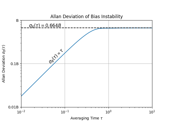
From the plot, we can see that there is a region where the Allan Deviation is proportional to \(\tau\). In this region, the flicker noise contributes very little to the deviation, so we can safely ignore it. We also see a flat region that converges to approximately \(0.664B\). So we can effectively approximate \(B\) from the plot by finding the flat region of the plot and dividing the Allan Deviation by 0.664.
At this point, the plots we’ve put together are of little help since we won’t be able to calculate the Allan Deviation plot for different sources of noise. In real life, these noise sources will be mixed and appear on the output of the IMU.
First, recall that we have assumed our sources of noise are statistically independent. As such, we can decompose the Allan Deviation of the entire noise spectrum into its constituent parts:
\(\sigma_{\eta}(\tau) = \sigma_N(\tau) + \sigma_B(\tau) + \sigma_K(\tau).\)
To analyze the total noise, we’ll simply add these Allan Deviations for some representative noise coefficients and plot the total Allan Deviation (\(N = 0.001, B = 0.0008, K = 0.00003)\).
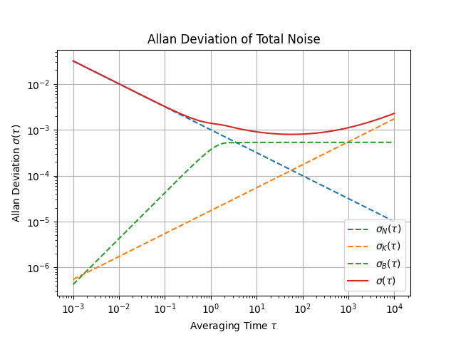
As seen in this plot, the same strategies as above can be taken to approximate our coefficients. To summarize
💡 In some cases, the Allan Deviation plot will take a V shape instead of a shallow bowl. In these cases, the total noise is dominated by white noise and brown noise. As such, modeling bias instability can be ignored for IMUs exhibiting this behavior.
For more information on this section and how to perform an Allan Deviation analysis refer to the IEEE Standard Specification for Gyroscopes (Annex C).
As mentioned earlier, the Allan Variance is typically calculated in fairly ideal conditions. As such, the parameters deduced in an Allan Variance analysis will only capture the effects of the latent noise in these same ideal conditions. So, it is common practice to inflate these estimated values to encompass additional unmodeled errors such as temperature fluctuations or other deterministic errors.
If you’d like help estimating the noise parameters of your IMU, or you’d like us to help you calibrate your IMU system, reach out! In our final post in this IMU series, we’ll talk about an efficient way to process IMU data — IMU Preintegration. If you’d like to be notified of when that next post drops, just follow us on LinkedIn, X, or subscribe to our newsletter. Don't have an IMU yet? Consider pre-ordering our upcoming HiFi depth sensor, for high-resolution 3D sensing...with a built-in IMU!